Towards a Meta-Language for the Concurrency Concern in DSLs (DATE’15)
Concurrency is of primary interest in the development of complex software-intensive systems, as well as the deployment on modern platforms. Furthermore, Domain-Specific Languages (DSLs) are increasingly used in industrial processes to separate and abstract the various concerns of complex systems. However, reifying the definition of the DSL concurrency remains a challenge. This not only prevents leveraging the concurrency concern of a particular domain or platform, but it also hinders: a) the development of a complete understanding of the DSL semantics; b) the effectiveness of concurrency-aware analysis techniques; c) the analysis of the deployment on parallel architectures. In this paper, we present MoCCML, a dedicated meta-language for formally specifying the concurrency concern within the definition of a DSL. The concurrency constraints can reflect the knowledge in a particular domain, but also the constraints of a particular platform. MoCCML comes with a complete language workbench to help a DSL designer in the definition of the concurrency within a DSL, and a generic workbench to simulate and analyze any model conforming to this DSL. MoCCML is illustrated on the definition of a simple DSL for signal processing, augmented with the specification of the deployment on different hardware platforms.
Overview
This page provides an overview of the steps to experiment on the SigPML DSL using MoCCML. The user will require downloading the above framework and source projects (Part 1, 2) and following the simple steps described in Part 3, or in Part 4 where the experiment is captured in video. Finally, Part 5 presents a case study and some experiment results.
Part 1: Required environment for the experimentation
The SigPML experimentation was realized in the GEMOC Studio framework for: the MoCC modeling with MoCCML; the SigPML constraining; and the simulation of system models realized with SigPML using TimeSquare (already integrated in the GEMOC Studio). The exhaustive exploration activities were realized in “GEMOC Studio” and “ClockSystem” which is in the process of being integrated in the GEMOC Studio. Here, we recommend using the GEMOC Studio exhaustive exploration facility and TimeSquare. To test the case study, the GEMOC Studio environment must be downloaded here.
Part 2: Source files for the experimentation
There are two categories of project files required for the experimentation. The first category of project files is related to the edition of the MoCC models and their mapping with the DSL. These activities are performed in the “language workbench”. The steps are illustrated later in Part 3. The second category of project files are related to the instance models representing the Passive Acoustic Monitoring system models and the MoCC-aware instance models for simulation in TimeSquare and exhaustive exploration in GEMOC Studio. The following links provide the sources: The “language workbench” project files (.zip) are available here. The “modeling workbench” projects file (.zip) is available here.
Part 3: Steps to realize the experimentation
All the steps are shown in the linked video of Part 4.
- Launch the GEMOC Studio
- Import the “language workbench” project files (used to define the SigPML DSL with the explicit MoCC definitions implemented in MoCCML)
- The SigPML project files (model, editor, etc.) are in:
- org.gemoc.sigpml.model
- org.gemoc.sigpml.model.design
- org.gemoc.sigpml.model.edit
- org.gemoc.sigpml.model.editor
- The MoCCML model (file extension= .mocc) files are in:
- org.gemoc.sigpml.moc.lib/MoCLib
- The mapping files (file extension= .ecl) between the MoCC models and the SigPML concepts are in:
- org.gemoc.sigpml.moc.application/MoCApplication
- The SigPML project files (model, editor, etc.) are in:
When changes are made and saved in the .ecl files a new file (.qvto) is generated and stored in org.gemoc.sigpml.moc.application/qvto-gen. This file will be used in the modeling environment to generate the MoCC-aware instance models.
- Launch a new GEMOC studio to enable the Modeling environment (new Eclipse Application)
- Import the “modeling workbench” project files (containing instances of SigPML models with MoCC properties)
- The Passive Acoustic System models are in:
- org.gemoc.sigpml.simple_example/DateExample
- The .qvto files are in:
- org.gemoc.sigpml.simple_example/QVTO_files
- The Passive Acoustic System models are in:
- All the instance models are stored in the directories PAM_0, PAM_1, PAM_2, PAM_3
- Models can be visualized using the .sigpml file
- Or graphically running the .aird file
- In order to Simulate the models:
- Create the MoCC-aware instance models for TimeSquare: right click on the .sigpml file, GEMOC -> Generate extended CCSL (Choose QVTO) -> select the qvto generated from the .ecl. An instance model is generated with extension (.extendedCCSL)
- Use the .extendedCCSL file to launch simulation: right click on the file -> Run AS -> CCSL Simulation (see video)
- Choose the number of simulation steps and the Simulation policy: Maximum(one of the solution)
- Activate VCD Generation
- Add the events to display
- Run the simulation
- Traces can be organized from the top Menu VCD Editor/ Clocks/Ordering (see video)
- Similar steps can be performed on the other .sigpml files.
- In order to realize exhaustive exploration of the state space:
- right click on the .extendedCCSL -> TimeSquare -> Compute State Space
Part 4: Video Description of the Experiment
Part 5: Case Study and Experimentation results
Click on the Figures to enlarge.
Case Study: a Passive Acoustic Monitoring (PAM)
The system is a Passive Acoustic Monitoring (PAM) system realized using SigPML (see Figure AgentSystemModel). Such system is used to survey and study underwater environment signals (noises from cetaceans or dolphins, etc.). One of the main issues for a PAM system is the transient signal detection in a continuous noise that is measured by a hydrophone (acquisition part of the smart sensor). Each sensor is based on signal processing algorithms coupled with hydrophones to process and interpret the raw data of the sensor.
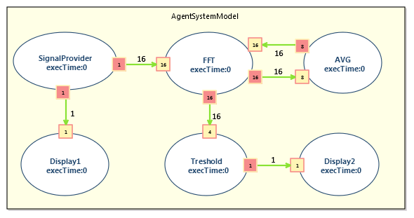
The PAM system is composed of six agents: Signal Provider, FFT, AVG, Threshold, Display1 and Display2. When activated, the Signal Provider produces 1 data; the FFT consumes data by 16 and transforms them into a time-frequency representation processed by AVG and Threshold to overcome the variations of the data on a long time interval. AVG consumes the data by 8 and performs an average “high-pass filter” with a feedback effect to the FFT. Finally Threshold processes data by 4. The MoCC applied to this example follows an SDF-like semantics as presented in the paper. There are two main MoCC constraints applied respectively on the Places and the Agents (see paper). In the following part, we present some of the results from experimenting MoCCML and SigPML with the PAM example.
Some Experiment Results on the Passive Acoustic Monitoring (PAM)
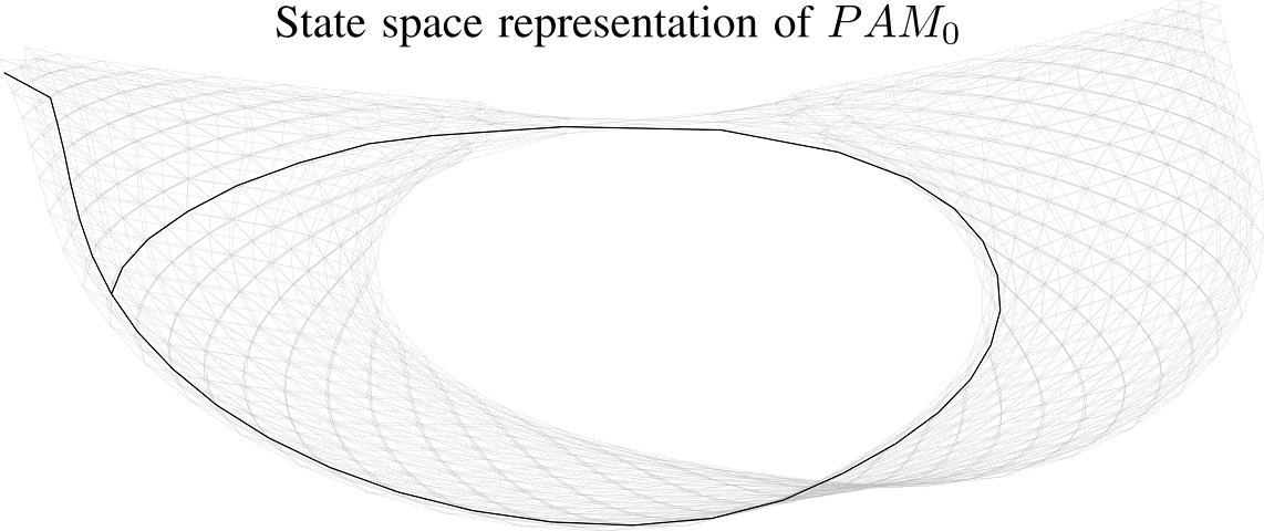
The execution model resulting from using MoCCML and SigPML for PAM modeling can be used by a generic execution engine either to simulate the system or to explore exhaustively all acceptable schedules. The exploration of all schedules can be captured explicitly in a state space graph as the one presented in Figure (State space representation of PAM0).
Figure (State space representation of PAM0) shows a graphical representation of the set of available schedules of the PAM application, under an infinite resource assumption (referred to as PAM0). The black line in the figure emphasizes the schedule that is obtained under ASAP simulation policy.
Any cyclic path in this graph (starting from the initial configuration) represents a valid schedule of the model.
The experimentations were also done considering platform allocations as shown in the table (Deployment strategies on 3 different platforms). We have tested 3 different allocation strategies for PAM0. These allocations correspond to a platform with: one computing resource (P1) in PAM1, four computing resources (P1..4) in PAM2, and two computing resources (P1,2) in PAM3. The PAM3 allocation model is shown in the below Figure (AgentSystemModel with allocation on cpu1, cpu2).
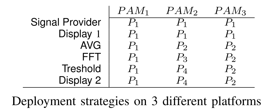
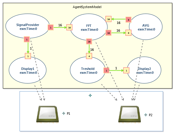
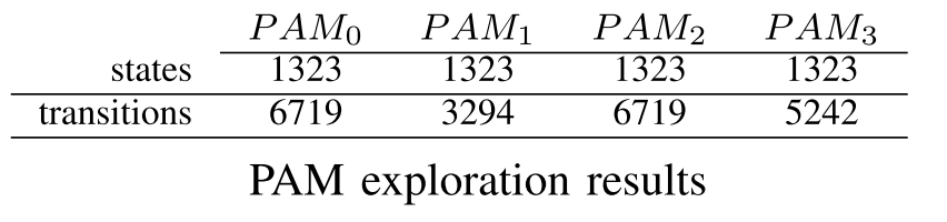
Table (PAM exploration results) shows some metrics on the number of states and transitions on each of the state-spaces resulting from the execution model of PAM in SigPML (without platform allocation i.e. PAM0, and with platforms allocations i.e. PAM1–PAM2–PAM3).
PAM3 represents a potentially better deployment of the agents since the schedule is like the one of PAM0 when only two processors are used. Indeed, PAM3 doesn’t have the infinite resource assumption made for PAM0, neither the sequential nature of PAM1, nor the 4 Processor allocation of PAM2 that generates more transitions in the state space.